5 Image post processing
5.1 File names and storage
We found that it is critical to have a very organized structure for saving files, especially when several people are working on the same project. We propose here what has been working so far for us.
In a species folder named with the name of the species (Genus_species), there should be a distinct folder for each individual photographed, usually with a different collection number. If the same individual has been photographed several times, the date of photos acquisition should be appended to the folder name to discriminate them. We also indicate in the folder name whether the individual has been photographed with or without sepals.
For each flower, we have one folder for uncalibrated photos, one for calibrated photos, and one for the model. The RAW picture of the color chart should be placed in the uncalibrated photos.
To distinguish which photo goes in which chunk, a photo of the label is taken at the beginning of each chunk (each set of photos per side of flower). We suggest to place the photos from different chunks in different folders once the photos are calibrated. The date of when the photos are taken is important because it helps matching the calibration to the right DNG file. If more than one set of photos with different lighting or camera settings are taken, make sure to distinguish the color charts that correspond to each set of photos.
Genus_species
GEN_species_CollectionNumber
sepal_DD.MM.YYYY or no_sepals_DD.MM.YYYY
Model
MetashapeProject
MetashapeProjectFolder.files
model.obj
model.ply
texture.jpg
01_Photos_to_calibrate
Place here all the RAW photos and color chart
02_Photos_calibrated
Place here all the calibrated photos, that you can organize per chunk
If you are doing focus stacking, you can also create the following two folders in addition to the above:
03_Photos_clustered
Place here the calibrated photos that have been clustered based on time intervals into separate subfolders containing series of pictures taken using the Focus Bracketing function at each rotation point
04_Photos_focus_stacked
Place here all the final images after focus stacking
5.2 Image color calibration
5.2.1 Creating color profiles
We present here three ways to create camera profiles. The first one allows to manually check the automatic detection of the color chart, the second and third ones are fully automatic (on MacOS and windows respectively).
This does not linearize the photos. For further details on color calibration, read Troscianko and Stevens (2015).
Method 1 : Manual creation of color profiles
This method uses the Xrite ColorChecker Camera Calibration software and Adobe DNG converter software (Figure 5.1).
Create a new empty folder called DNG.
Copy the RAW file representing your color chart in your DNG folder, and rename it accordingly (e.g. Color_chart_DD.MM.YYYY).
Open DNG converter and select the DNG folder you created in the first step. You can’t select a specific file, you need to select a folder, and the software will convert all the files within this folder. Default parameters are fine for step 2-4. It will export the RAW file in the DNG folder to a DNG file with the same file name (Figure 5.2).
Open the Color Checker Camera Calibration software and drag and drop the newly created DNG file in the software. The software will automatically draw a grid around it. Make sure that the green grid fits the chart, avoiding edge effects on each square of color (Figure 5.3.
Click on Create Profile and save it under Color_Chart_DD.MM.YYYY (Figure 5.4.
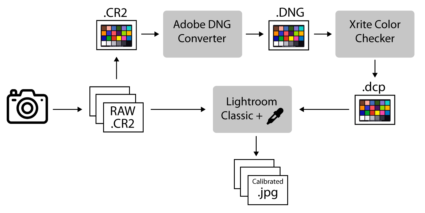
Figure 5.1: Image color calibration workflow.
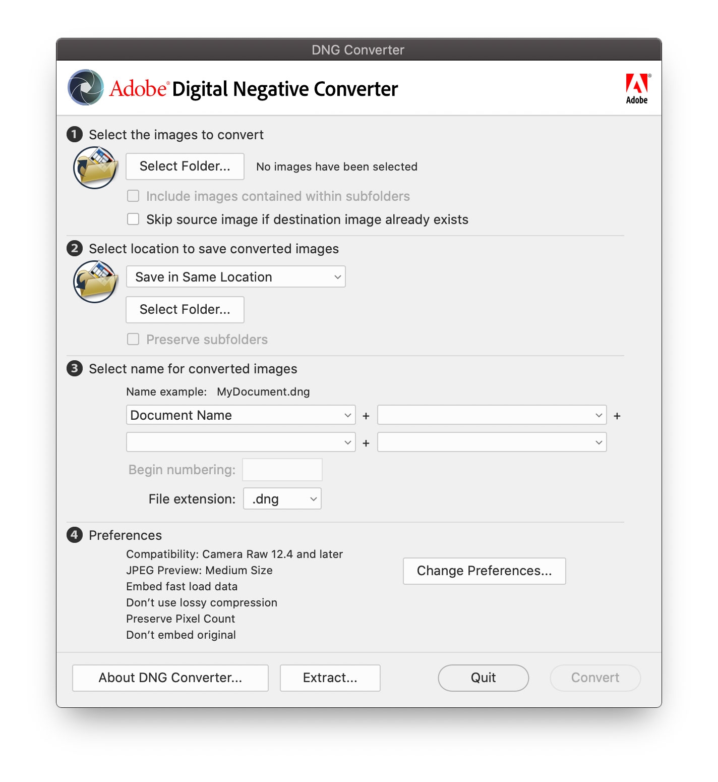
Figure 5.2: Convert RAW chart to DNG in Adobe DNG Converter.
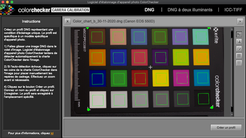
Figure 5.3: Align grid on chart in ColorChecker Camera Calibration.
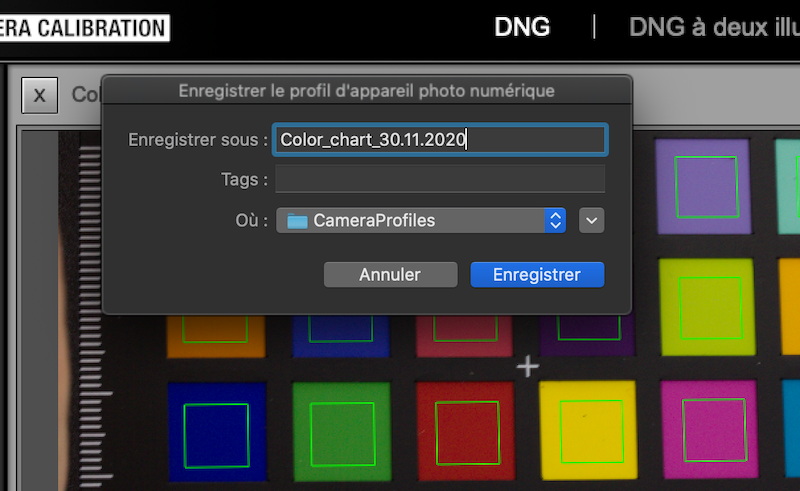
Figure 5.4: Export the color profile.
Method 2: X-Rite Color Checker plug-in installation and automatic creation of color profiles on MacOS
Directly in Adobe Lightroom, you can add ColorChecker Camera Calibration as a module to a means of exporting files directly into a color profile.
Click on File > Export > Plug-in Manager (or gestionnaire des modules externes in the left bottom corner).
Click on Add.
Navigate to Library > Application Support > Adobe > Lightroom > Modules.
Select XRiteColorCheckerPassport.lrplugin and then click on Add Plug-in and Done.
Click on the color chart then File > Export > Choose Xrite presets from the drop down menu.
Name your profile then > Export.
It will go through ColorCheckerCamera calibration to automatically create the profile.
Restart Lightroom as indicated.
Method 3: X-Rite Color Checker plug-in installation and automatic creation of color profiles on Windows
Get the Xrite ColorChecker Camera Calibration software and download the PC Version. Save the CameraCalibrationSetup.exe in your downloads, for example, and run the program.
If Adobe Lightroom Classic is already installed on your computer, the installation program should proposed you to install the Adobe Photoshop Lightroom plug-in (Figure 5.5). Install it.
Once the plug-in is installed, run Adobe Lightroom Classic and import your color chart (File > Import).
Click on File > Export and in the drop-down menu, select X-Rite Preselection (Figure 5.6). Name your profile, and click on Export.
Restart Lightroom as indicated.
Run the setps 4 and 5 each time you want to create a new color profile witht the color chart.
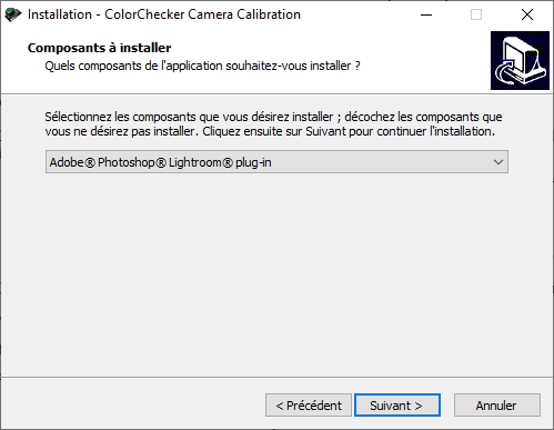
Figure 5.5: Color Checker plug-in for Lightroom installation.
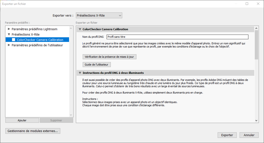
Figure 5.6: Color chart profile exportation.
5.2.2 Color and exposure calibration from profiles
Import your photos in Lightroom Classic. File > Import then select your folder of RAW photos.
Select the photo of the color chart.
Go to the Development module.
Select the color profile corresponding to the color chart you have selected (see Figure 5.7 and 5.8 to manually add a color profile) to calibrate the photo of the chart with its own calibration profile.
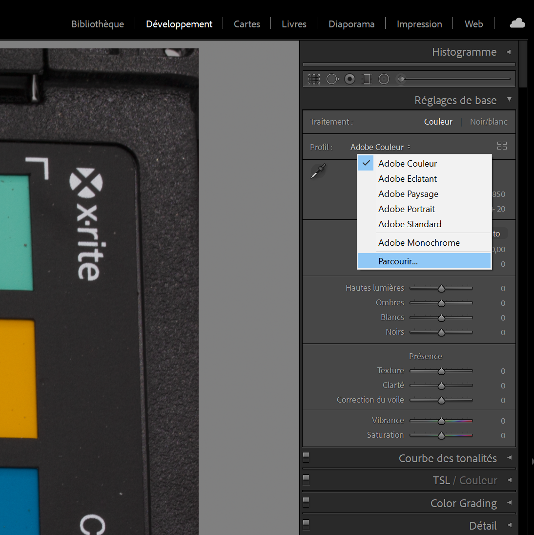
Figure 5.7: Add a new color profile.
Figure 5.8: After adding a profile with the + sign, select it in the list below.
Use the eyedropper over the 75% gray scale (the dark gray patch right before the black patch on the color chart). Do not click on the photo with the eye dropper, only hover over it.
Adjust the RGB values the eyedropper indicates on the 75% gray scale by changing the exposure setting to make them as close as possible to 0.33 0.33 0.33 (corresponding to 85/255 for each of the red, blue, and green class). The exposure is now adjusted in addition to the color calibration, but only on the chart image.
To apply the modifications we just did to all the photos, go to the Library module, select all the photos (Cmd+A or Ctrl+A), and make sure that the one for which you made changes is highlighted (in white compared to the light gray of the newly selected images).
Go back to the Development module and click on the Synchronize option, check the profile and exposure boxes in the pop-up window and click on Synchronize (see Figure 5.9).
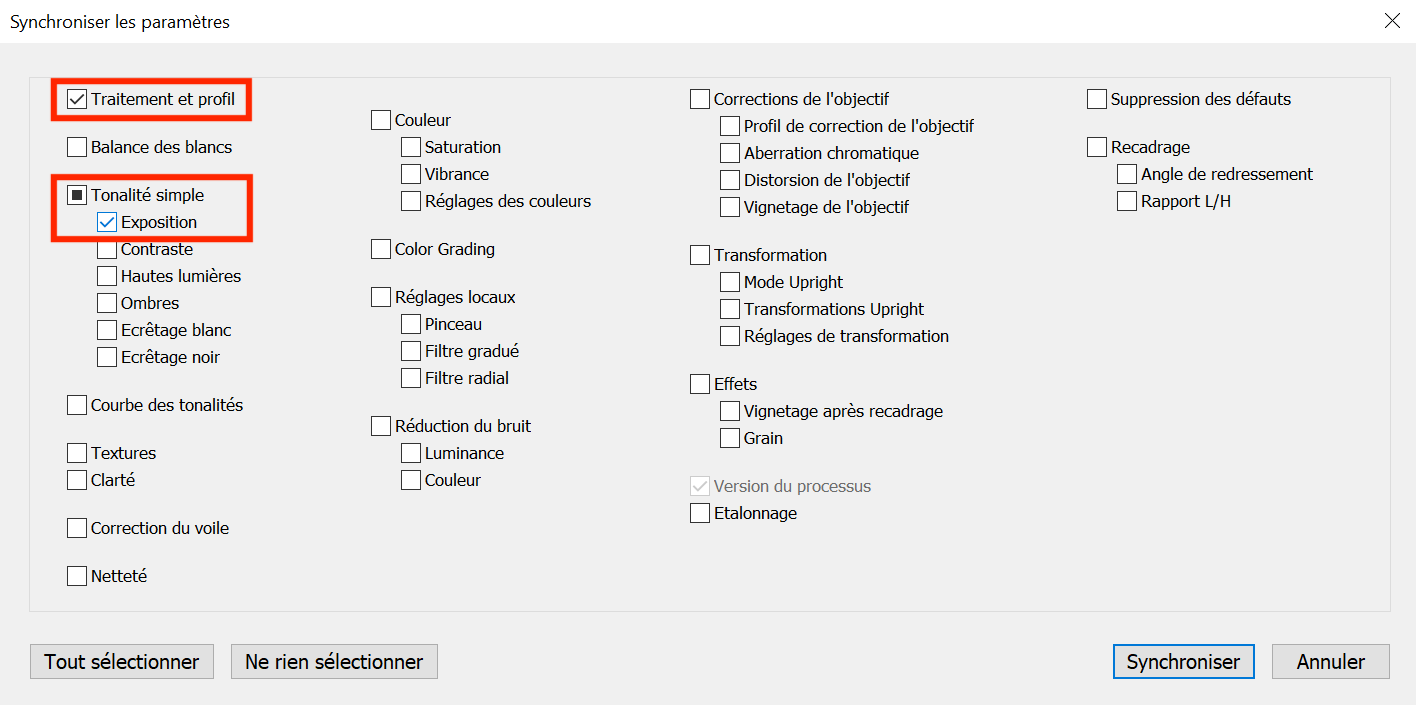
Figure 5.9: Synchronize your settings made to the photo of the chart to all the other photos and check the two categories you modified (color profile and exposure).
5.2.3 Export calibrated files
Select all the photos you need to export or all of them (Cmd+A or Ctrl+A).
Click on File > Export.
You can create presets that you will only need to create once to always export the same way in Adobe Lightroom (example Figure 5.10), and add personalized file names such as "_color_calibrated" at the end of each image file.
- Without focus stacking: Save the calibrated images as JPEG.
- With focus stacking: Save the calibrated images as TIFF (300 PPI). Make sure to include all metadata.
The calibrated folders can be saved into their own folder, and further divided into different subfolders representing different chunks (easily distinguishable by the separation created by a photo of the label).
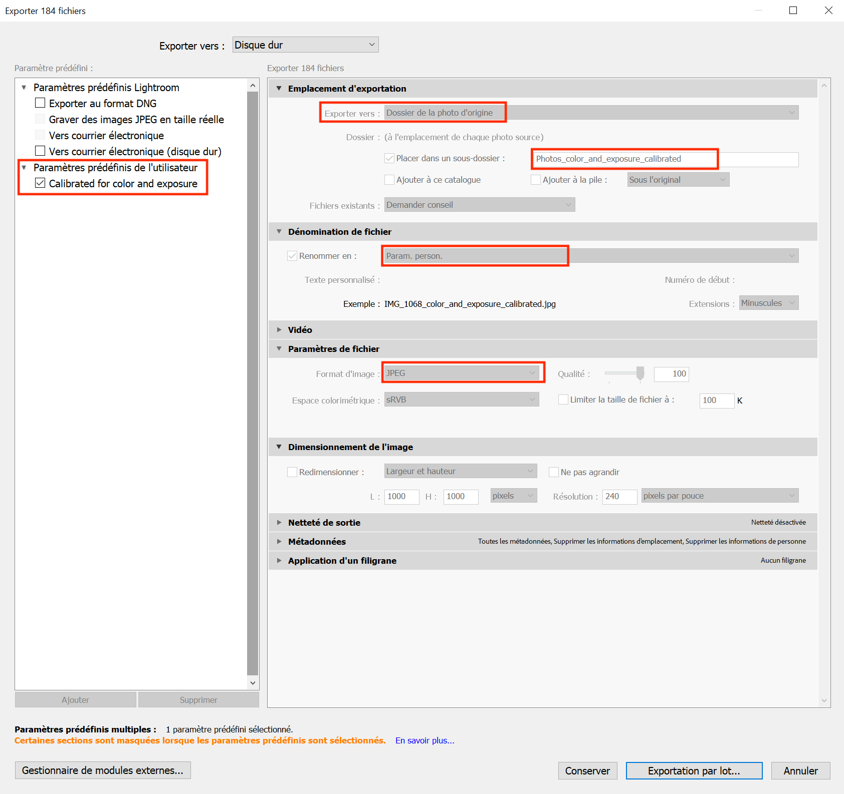
Figure 5.10: You can export using your own personalized parameters and then export in batch your selection in a specific folder within your folder of uncalibrated photos for easy access. This method can thus work for any folder of uncalibrated photos.
5.3 Image clustering (one folder at a time)
Note: This step is only necessary if you chose to do focus stacking in your project.
If you used the Focus Bracketing function during image capture and wish to proceed with focus stacking, you can make the process easier by first grouping (i.e., clustering) the series of photos taken at each angle and rotation point in separate subfolders. This way, each folder will contain images that can be stacked together as they depict the same flower angle and rotation point but with different focus distances.
This can be achieved using ExifTool. ExifTool extracts time-stamps from the metadata of images and can be used to separate the image clusters from each other based on time intervals. The time intervals between photos taken at each rotation point (i.e., at the same exact perspective, but with different focus distances) is smaller than between photos taken between two rotation points (i.e., after the turntable changes the flower angle) when using the Focus Bracketing function.
To make image clustering faster, a python script developed by the Eaton Lab can be used (cluster_photos_by_time_intervals.py).
Command structure:
python3 cluster_photos_by_time_intervals.py -i <input folder with calibrated images> -o <output folder with clustered images>Example:
python3 cluster_photos_by_time_intervals.py -i 02_Photos_calibrated -o 03_Photos_clusteredAfter running the command above, you will have a 03_Photos_clustered folder containing subfolders with the different
image clusters, distinguished by angle and rotation numbers based on their time-stamps.
5.4 Focus stacking (one folder at a time)
Note: This step is only necessary if you chose to do focus stacking in your project.
With the image groups taken at each rotation point and angle separated into different folders, they can now be easily focus stacked to produce one image per cluster with the whole flower in focus. Similarly to image clustering, this can be achieved by running another python script developed by the Eaton Lab (helicon_focus.py).
Command structure:
python3 helicon_focus.py -i <input folder with clustered images> -o <output folder with focus stacked images>Example:
python3 cluster_photos_by_time_intervals.py -i 03_Photos_clustered -o 04_Photos_focus_stackedNow you should have a 04_Photos_focus_stacked folder containing one focus
stacked image corresponding to each angle and rotation point cluster.
5.5 Alternatively: Cluster and focus stack photos from multiple folders at once
In case you would like to cluster and focus stack images of multiple specimens at once, to make the process even faster, you could also use the Automated Pipeline Scripts developed by the Eaton Lab.
You can use these scripts for all steps (i.e., from image calibration to focus stacking) or modify them according to your preferences and needs. We normally do the calibration step manually in Adobe Lightroom Classic as it does not take significantly more time and allows for calibrating both the colors and exposure of the images.
To make the scripts work, we save the calibrated images in a subfolder directly in
the corresponding RAW image folder, for example in 3D_Modelization/Genus_species_A/01_Photos_calibrated/,
with the RAW images being in 3D_Modelization/Genus_species_A/, while the directory containing the
3D_Modelization/ contains other folders that are similarly structured for other species.
3D_Modelization
Genus_species_A
RAW_photo_A1.CR3
RAW_photo_A2.CR3
RAW_photo_A3.CR3
…
01_Photos_calibrated
Calibrated_photo_A1.tif
Calibrated_photo_A.tif2
Calibrated_photo_A3.tif
…
Genus_species_B
RAW_photo_B1.CR3
RAW_photo_B2.CR3
RAW_photo_B3.CR3
…
01_Photos_calibrated
Calibrated_photo_B1.tif
Calibrated_photo_B2.tif
Calibrated_photo_B3,tif
…
…
For the sake of simplifying the following examples,3d_Modelization/ would represent the path to your working directory that contains all your folders.
First, you need to create a text file containing a list of folder names in your
working directory, i.e., the folders names in the directory 3D_Modelization/
following the example above. cd to this directory and run the following command:
ls -b1A >> folder_name.txtThis command will create a folder_name.txt file in your working directory with the names of
all the folders in it. Then you need to create a text file containing the list of
the RAW photo names within these folders.
Command structure:
for i in `cat folder_name.txt`; do cd 3D_Modelization/${i} && ls *.CR3 | sed -e 's!.CR3!!' >> photo_names.txt; done
Now, aside from the RAW photos and the subfolder with the calibrated .tif photos,
the Genus_species_#/ folders within the 3D_Modelization/ directory should contain
a photo_names.txt file with a list of the names of all the RAW photos in each folder.
We usually run the following modified automated script for processing multiple folders at once.
- Automated script structure for clustering and focus stacking photos from multiple folders at once:
for i in `cat 3D_Modelization/folder_name.txt`
    do python3 cluster_photos_by_time_intervals.py -i 3D_Modelization/${i}/01_Photos_calibrated -o 3D_Modelization/${i}/02_Photos_clustered &&
    python3 helicon_focus.py -i 3D_Modelization/${i}/02_Photos_clustered -o 3D_Modelization/${i}/03_Photos_focus_stacked
done
The for loop above should create two new subfolders in each of
your 3D_Modelization/Genus_species_#/ directories:
02_Photos_clustered, containing the calibrated photos that have been clustered by angle and rotation points based on time intervals.03_Photos_focus_stacked, containing the final focus stacked photos.
Although the original automated pipeline script by the Eaton Lab includes a step for resizing the photos after focus stacking, we do not typically include this step in the process as the photos’ dimensions before and after focus stacking remains the same most of the time. Additionally, changing the images’ dimensions to a different ratio can distort the shape of your 3D Model.
For those few images whose dimensions do change after focus stacking (for us it’s normally no more that 3 per specimen), during the masking step in Agisoft Metashape it will notify you that the background image you are using does not have the same size as some of the images. You can find those unmasked photos and create a background images using their dimensions for masking them. However, as mentioned, this happens rarely.
If you wish to resize all your images after focus stacking following the original script,
you will need to install imagemagick, which could be done using homebrew.
brew install imagemagick- Automated script structure for clustering, focus stacking, and resizing photos from multiple folders at once:
for i in `cat 3D_Modelization/folder_name.txt`
    do python3 cluster_photos_by_time_intervals.py -i 3D_Modelization/${i}/01_Photos_calibrated -o 3D_Modelization/${i}/02_Photos_clustered &&
    python3 helicon_focus.py -i 3D_Modelization/${i}/02_Photos_clustered -o 3D_Modelization/${i}/03_Photos_focus_stacked &&
    cd 3D_Modelization/${i}/03_Photos_focus_stacked && ls -b1A | sed -e 's!.tiff!!' >> stacking_names.txt &&
    for i in `cat stacking_names.txt`
        do convert ./${i}.tiff -resize 5300x3500! ./${i}.tiff
    done
done
Remember to add the path to your python script files if they are not located in your working directory, as well as modify the final image size if you wish it to be different.